1 - Basics
1.1 - Models
Kinetic models are at the heart of S-timator. These models are conceptual descriptions of real systems that are characterized by stating the rates of change of entities.
Generically, a kinetic model is a set of processes that produce or consume several variables. Variables are required to be associated with a value of amount or concentration.
Examples of processes, from various scientific fields, are:
- a chemical reaction
- the flow of charge in a node of an electrical network
- predation in an ecological system
- the inflow of potassium into the axon of a neuron
Processes are related to change, transport or transformation.
Examples of variables are:
- the concentrations of a chemical species
- the number of individuals in the population of prey
- the charge of a capacitor
- the ammount of mRNA transcribed from a gene.
A key requirement in the formulation of a kinetic model is that the rate the processes is known or can be assigned in advance. These rates usually depend on the concentrations of variables and, in turn, affect the concentrations of the variables that are “connected” by them.
But modelling (the act of formulating a model) is not about the study of the kinetics of the individual processes.
Instead, the primary objective is to predict or make inferences about the dynamics of the system as a whole, in particular to predict the change in the concentrations of the variables considered in the model.
To keep it simple, let’s start by looking at the following system of two chemical reactions:
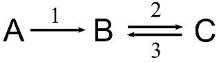
Example: a two-reaction chemical system
This reaction scheme indicates that a chemical species A is transformed into B by reaction 1 and, in turn, B is transformed into C by reaction 2. The arrows mean that reaction 1 is almost irreversible, whereas reaction 2 is reversible.
If we consider that the reactions are *processes* and the concentrations of the chemical species are the *variables*, we are starting to formulate a kinetic model about this system.
As stated before, a requirement is that the we must indicate the rates of the two reactions.
In simple chemical reactions, if the temperature is approximately constant, it is usually assumed that the rates of the individual steps of the reactions have what is called mass-action kinetics. In this example, the rates of the reactions would be:
Here, \(v_1\) and \(v_2\) represent the rates of the reactions 1 and 2, respectively, \(A\), \(B\) and \(C\) represent the concentrations of the chemical species and \(k_1\), \(k_2\) and \(k_3\) are constants appearing in the mathematical expressions of the rates. These constants are called parameters of the model.
The values of the parameters must also be indicated in a kinetic model:
At the bare minimum, a kinetic model is built by stating:
- how the variables are connected by the processes
- the rates of the processes (how do they depend on the variables)
- the values of the parameters that appear in the mathematical expression of the rates.
1.2 - Describing models in S-timator
How can we use S-timator to analyze this simple two-reaction example?
We must start by importing function read_model() from the S-timator package.
As we will see in a moment, this is one of the most fundamental functions of the package.
from stimator import read_model
#%matplotlib inline
In S-timator, models are described inside a Python string:
model_description = """

title A two-reaction chemical system

r1: A -> B, rate = k1 * A
r2: B -> C, rate = k2 * B - k3 * C

k1 = 0.1
k2 = 2
k3 = 1

init: (A = 1)

"""
This (multi-line) Python string contains a set of declarations about the model that are quite straightforward to learn and use.
Let us examine them:
The title is a line is that begins with the word title and is supposed to contain a small description of the model.
The processes are lines that describe the processes by indicating the “stoichiometry” of the the processes (that is, how they connect the variables of the model) and the rates of those processes. In this example, consider the line
r1: A -> B, rate = k1 * A
The format of these lines is: the name of the process (r1), followed by a collon, followed by the “stoichiometry” of the process (“A -> B”) followed by a comma and a statement of the rate (“rate = k1 * A”). So, this line says that reaction r1 transforms A into B with rate k1 *A.
The parameters are lines that indicate the values of the parameters of the model. The format is, simply, the name of the parameter, followed by an equal sign, followed by the value of the parameter.
The initial state is a line that starts with init:, followed by a list of values for the variables of the model. These values are supposed to prescribe a state of the model that can serve as an initial (multi-dimensional) starting point from which the dynamics of the system evolves. More about this ahead. In this example, we are setting a value of 1 for variable A. The other variables, B and C will be zero, the default.
Note that, in this example, reaction 1 was named r1 and the reactions 2 and 3 are considered the forward and backward steps of reaction r2.
After writting the string that describes the model, this string must be transformed into a special Python object using function read_model().
The result of read_model() is a ``Model`` object, one of the fundamental data structures in S-timator.
Model objects expose a lot of functionality realted to the computational study of kinetic models.
m = read_model(model_description)
We can print a Model object, generating a small report of the components of the model.
print m
Just a few notes:
- Variables are not declared: they are infered from the “stoichiometry” of the processes.
- Processes must be given a name. Many things that you can do with a Model depend on that. In this example, the two reactions were called “r1” and “r2”. Names must begin with a letter and can not have spaces. (we could not have given the names “1” and “2” to the two reactions).
- The “rate =” part in the declarations of the processes can be dropped: we could just have written “r1: A -> B, k1 * A” for reaction r1.
1.3 - Solving and plotting
One of the most basic procedures that one can do with a model is to “solve” it and then plot the results.
Two functions are involved:
- solve()
- plot()
m.solve(tf=20.0).plot()
Where did this graph came from?
S-timator took the initial state of your model, as defined in init, and generated an estimate of the values of the concentrations of the variables throughout time. This is called a time course or a time series.
Function plot() just produces a graph of those values, where the x-axis represents time.
The two functions were chained together: the result of solve() can call the function plot() just by using the dot.
Why is it called solve()?
This is because the underlying mathematical expression of the model is a system of ordinary differential equations (SODE).
For our two-reaction example, this system is
Computing the time course of the concentrations, starting from the initial state, is done by solving this system of equations numerically, that is, computing \(A(t)\), \(B(t)\) and \(C(t)\) as functions of time, from the knowledge of their derivatives. Hence the name solve().
The result of function solve() is called a solution of the SODE.
The argument tf in function solve() indicates that the solution should be computed up to the value of tf.
Let’s change this value
s = m.solve(tf=100.0)
s.plot()
Here the two functions, solve() and plot() were separated. The result of solve() (a time course) was assigned to the variable s and then s.plot() was called.
Looking at the plot, we can see that, given enough time, species \(A\) is completely consumed and the total mass (1.0) is distributed among \(B\) and \(C\), which settle into a chemical equilibrium.
We can obtain the final values of the time course, using attribute last of the solution object:
s.last
last is returned as a Python dictionary.
1.4 - Inflows and outflows
Let’s consider another example, similar to the two-reaction chemical system.
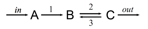
Example: a two-reaction open chemical system
In this example, there are two aditional “reactions”: an inflow of \(A\) into the system and an outflow of \(C\) out of the system. These could represent a continuous feed of new substrate \(A\) in a chemical reactor and the precipitations of \(C\) into a solid salt.
How do we describe those types of processes from or into the “exterior” of the system in S-timator?
Simply, those processes have an empty left or right side in their stoichiometry:
model_description = """
title An open two-reaction chemical system

inflow: -> A, rate = kin
r1: A -> B, rate = k1 * A
r2: B -> C, rate = k2 * B - k3 * C
outflow: C ->, rate = kout * C

kin = 0.5
k1 = 0.1
k2 = 2
k3 = 1
kout = 0.2

init: (A = 0, B = 0, C = 0)
"""

m = read_model(model_description)
Repeating the analysis for this example, we get very different results.
s = m.solve(tf=100.0)
print s.last
s.plot()
Here the three variables settle into a different state characterized by the steady flow of mass throughout the system (a steady state). Notice that \(A\) no longer vanishes to zero.
It is also interesting to plot the rates of the four reactions. We can achieve this by using argument outputs of function solve(): the “glyph” -> indicates that the rates should be computed, instead of the variables (>> or > could also have been used).
s = m.solve(tf=100.0, outputs='->')
print s.last
s.plot(yrange=(0,0.6))
Not only the concentrations become constant but the values of the rates also become constant and equal to the inflow of mass into the system.