2 - More on models and model description¶

This chapter will focus on the “mini-language” used to describe models in S-timator and also on the model objects created by function read_model()

from stimator import read_model

Picking up the last example from the previous chapter: the open two-enzyme system:

Example: a two-reaction open chemical system

Recall that the minimum components of a model declaration are:

title
reactions
parameters
init

model_description = """
title An open two-reaction chemical system

inflow: -> A, rate = kin
r1: A -> B, rate = k1 * A
r2: B -> C, rate = k2 * B - k3 * C
outflow: C ->, rate = kout * C

kin = 0.5
k1 = 0.1
k2 = 2
k3 = 1
kout = 0.2

init: (A = 0, B = 0, C = 0)
"""

m = read_model(model_description)

print m

An open two-reaction chemical system

Variables: A B C

inflow:
  reagents: []
  products: [('A', 1.0)]
  stoichiometry: ->  A
  rate = kin

r1:
  reagents: [('A', 1.0)]
  products: [('B', 1.0)]
  stoichiometry: A ->  B
  rate = k1 * A

r2:
  reagents: [('B', 1.0)]
  products: [('C', 1.0)]
  stoichiometry: B ->  C
  rate = k2 * B - k3 * C

outflow:
  reagents: [('C', 1.0)]
  products: []
  stoichiometry: C ->
  rate = kout * C

init: (A = 0.0, C = 0.0, B = 0.0)

k3 = 1
k2 = 2
k1 = 0.1
kin = 0.5
kout = 0.2

2.1 - Reactions¶

You can iterate over the reactions of a model:

for v in m.reactions:
    print (v)

inflow:
  reagents: []
  products: [('A', 1.0)]
  stoichiometry: ->  A
  rate = kin

r1:
  reagents: [('A', 1.0)]
  products: [('B', 1.0)]
  stoichiometry: A ->  B
  rate = k1 * A

r2:
  reagents: [('B', 1.0)]
  products: [('C', 1.0)]
  stoichiometry: B ->  C
  rate = k2 * B - k3 * C

outflow:
  reagents: [('C', 1.0)]
  products: []
  stoichiometry: C ->
  rate = kout * C

Or, just to get the names:

for v in m.reactions:
    print (v.name)

inflow
r1
r2
outflow

A reaction has a lot of attributes:

v = m.reactions.r1
print (v.name)
print (v.reagents)
print (v.products)
print (v.stoichiometry_string)
print (v.stoichiometry)
print (v())

r1
[('A', 1.0)]
[('B', 1.0)]
A ->  B
[('A', -1.0), ('B', 1.0)]
k1 * A

Model.varnames is a list of variable names and Model.parameters can be used to iterate over the parameters of a model.

print (m.varnames)
for p in m.parameters:
    print ('%6s = %g' % (p.name, p))

['A', 'B', 'C']
    k3 = 1
    k2 = 2
    k1 = 0.1
   kin = 0.5
  kout = 0.2

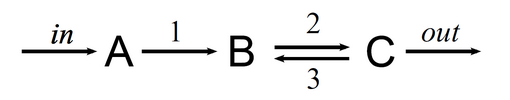
2.2 - Transformations¶

Transformations are declared starting a line with a ~. These are quantities that vary over time but are not decribed by differential equations. In this example total is a transformation.

model_description = """
title An open two-reaction chemical system

inflow: -> A, rate = kin
r1: A -> B, rate = k1 * A
r2: B -> C, rate = k2 * B - k3 * C
outflow: C ->, rate = kout * C

kin = 0.5
k1 = 0.1
k2 = 2
k3 = 1
kout = 0.2

init: (A = 0, B = 0, C = 0)

~ total = A + B + C
"""

m = read_model(model_description)
print m

An open two-reaction chemical system

Variables: A B C

inflow:
  reagents: []
  products: [('A', 1.0)]
  stoichiometry: ->  A
  rate = kin

r1:
  reagents: [('A', 1.0)]
  products: [('B', 1.0)]
  stoichiometry: A ->  B
  rate = k1 * A

r2:
  reagents: [('B', 1.0)]
  products: [('C', 1.0)]
  stoichiometry: B ->  C
  rate = k2 * B - k3 * C

outflow:
  reagents: [('C', 1.0)]
  products: []
  stoichiometry: C ->
  rate = kout * C

total:
  rate = A + B + C

init: (A = 0.0, C = 0.0, B = 0.0)

k3 = 1
k2 = 2
k1 = 0.1
kin = 0.5
kout = 0.2

m.solve(tf=50.0, outputs=["total", 'A', 'B', 'C']).plot(show=True)

2.3 - Local parameters in processes¶

Parameters can also “belong”, that is, being local, to processes.

In this example, both r1 and r2 have local parameters

Notice how thes paraemters are listed and refered to in print m:

model_description = """
title An open two-reaction chemical system

inflow: -> A, rate = kin
r1: A -> B, rate = k * A, k = 0.1
r2: B -> C, rate = kf * B - kr * C, kf = 2, kr = 1
outflow: C ->, rate = kout * C

kin = 0.5
kout = 0.2

init: (A = 0, B = 0, C = 0)

~ total = A + B + C
"""

m = read_model(model_description)
print m

An open two-reaction chemical system

Variables: A B C

inflow:
  reagents: []
  products: [('A', 1.0)]
  stoichiometry: ->  A
  rate = kin

r1:
  reagents: [('A', 1.0)]
  products: [('B', 1.0)]
  stoichiometry: A ->  B
  rate = k * A
  Parameters:
    k = 0.1

r2:
  reagents: [('B', 1.0)]
  products: [('C', 1.0)]
  stoichiometry: B ->  C
  rate = kf * B - kr * C
  Parameters:
    kr = 1
    kf = 2

outflow:
  reagents: [('C', 1.0)]
  products: []
  stoichiometry: C ->
  rate = kout * C

total:
  rate = A + B + C

init: (A = 0.0, C = 0.0, B = 0.0)

kin = 0.5
kout = 0.2

But this model is exactly the same has the previous model. The parameters were just made local. (plot() produces the same results).

m.solve(tf=50.0, outputs=["total", 'A', 'B', 'C']).plot()

The iteration of the parameters is now different:

for p in m.parameters:
    print p.name, p

kin 0.5
kout 0.2
r1.k 0.1
r2.kr 1.0
r2.kf 2.0

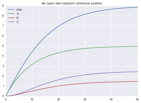
2.4 - External variables¶

An external variable is a parameter that appears in the stoichiometry of a reaction. It is treated as a constant.

In this example, D is an external variable:

m = read_model("""
title An open two-reaction chemical system

inflow: D -> A, rate = kin * D
r1: A -> B, rate = k * A, k = 0.1
r2: B -> C, rate = kf * B - kr * C, kf = 2, kr = 1
outflow: C -> E, rate = kout * C

D = 1
kin = 0.5
kout = 0.2
E = 2

init: (A = 0, B = 0, C = 0)

~ total = A + B + C
""")
print m

An open two-reaction chemical system

Variables: A B C

External variables: D E

inflow:
  reagents: [('D', 1.0)]
  products: [('A', 1.0)]
  stoichiometry: D ->  A
  rate = kin * D

r1:
  reagents: [('A', 1.0)]
  products: [('B', 1.0)]
  stoichiometry: A ->  B
  rate = k * A
  Parameters:
    k = 0.1

r2:
  reagents: [('B', 1.0)]
  products: [('C', 1.0)]
  stoichiometry: B ->  C
  rate = kf * B - kr * C
  Parameters:
    kr = 1
    kf = 2

outflow:
  reagents: [('C', 1.0)]
  products: [('E', 1.0)]
  stoichiometry: C ->  E
  rate = kout * C

total:
  rate = A + B + C

init: (A = 0.0, C = 0.0, B = 0.0)

E = 2
kout = 0.2
D = 1
kin = 0.5

m.solve(tf=50.0, outputs=['A', 'B', 'C', 'D', 'E']).plot()

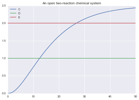
2.5 - Declaration of outputs¶

You can use !! to specify what should go into the solution of the model:

m = read_model("""
title An open two-reaction chemical system

inflow: D -> A, rate = kin * D
r1: A -> B, rate = k * A, k = 0.1
r2: B -> C, rate = kf * B - kr * C, kf = 2, kr = 1
outflow: C -> E, rate = kout * C

D = 1
kin = 0.5
kout = 0.2
E = 2

init: (A = 0, B = 0, C = 0)

~ total = A + B + C

!! C D E
""")
m.solve(tf=50.0).plot()

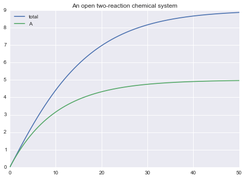
Or use the outputs argument to the solve() function (in the form of a list of desired outputs):

m.solve(tf=50.0, outputs=['total', 'A']).plot()

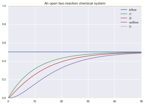
-> can be used to specify the values of all the rates of all the processes.

m.solve(tf=50.0, outputs=['->', 'D']).plot()

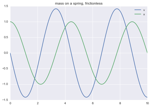
2.6 - Explicit differential equations¶

m = read_model("""
title mass on a spring, frictionless

# F = m * a = m * v' = - k * x
# by Hooke's law and Newton's law of motion

v' = -(k * x) / m
x' = v

m = 0.5
k = 1

init: x = 1
""")
m.solve(tf=10.0).plot()

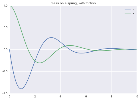
m = read_model("""
title mass on a spring, with friction

# using Hooke's law and friction proportional to speed,
# F = m * a = m * v' = - k * x - b * v

v' = (-k*x - b*v) / m
x' = v

m = 0.5
k = 1
b = 0.5

init: x = 1
""")
m.solve(tf=10.0).plot()

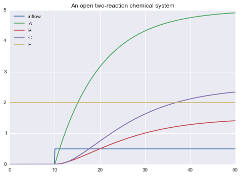
2.7 - Forcing functions¶

m = read_model("""
title An open two-reaction chemical system

inflow: D -> A, rate = kin * D * step(t, 10, 1)
r1: A -> B, rate = k * A, k = 0.1
r2: B -> C, rate = kf * B - kr * C, kf = 2, kr = 1
outflow: C -> E, rate = kout * C

D = 1
kin = 0.5
kout = 0.2
E = 2

init: (A = 0, B = 0, C = 0)

!! inflow A B C E
""")
m.solve(tf=50.0).plot()